Global distributions of the naturalized alien flora

Welcome to Global Distributions of Naturalized Alien Flora

Explore the naturalized alien plants and their global distributions. Our web application provides a comprehensive platform to visualize and understand the geogrphical distribution of naturalized plant across the globe under current conditions and future environmental scenarios, a critical aspect of biodiversity research and conservation.

Objective

We aim to provide an accessible and valuable resource for researchers, environmental managers, policymakers, and anyone interested in the dynamics of biological invasions. By making this data and its visualizations readily available, we hope to foster a greater understanding of alien plant distributions and support informed decisions for environmental protection and biodiversity conservation.

How to use this platform

This platform is an extension of ongoing research on the global geography of plant invasion risk under future environmental change. We continuously update our data and models to reflect the latest scientific findings. Start your exploration by navigating through the sections:

• Research: An overview about the study, methods, and data sources
• Single Species Maps: Explore and visualize the geogrphical distribution of the 9,701 species
• Download: Download the raster data for each of these 9,701 species

---

The global geography of plant invasion risk under future environmental change, (Nature Ecology & Evolution)

Ali Omer^1,2, Stefan Dullinger³, Johannes Wessely³, Bernd Lenzner¹, Adrián García-Rodríguez¹, Anna Schertler¹, Dietmar Moser³, Andreas Gattringer³, Amy J.S. Davis⁴, Wayne Dawson⁵, Trevor Fristoe⁶, Matthias Grenié⁷, Nicole L. Kinlock⁴, Holger Kreft^8,9,10, Jan Pergl¹¹, Petr Pyšek^11,12, Mark van Kleunen^4,13,14, Patrick Weigelt¹⁵, Marten Winter¹⁶, Damaris Zurell¹⁷, Franz Essl¹

Authors Affiliations

---

Introduction

The increasing threat of plant invasions to global biodiversity has raised interest in assesing their fine-scale distributions worldwide. Using Species Distribution Models (SDMs) implemented in the ‘biomod2’ R package version 4.2-5-2 (Thuiller et al., 2024), we modeled the current and future potential distributions of 9,701 naturalized alien plant species (~70% of the global naturalized alien flora), until the end of the 21st century. We calibrated our models with two alternative sets of environmental predictors (Table 1) that are known to affect plant distribution. We used four modeling algorithms: two regression techniques (generalized linear models, GLM; general additive models, GAM), and two machine learning techniques (random forests, RF; boosted regression trees, BRT).
To project potential future distributions by 2100, we used the Shared Socioeconomic Pathways (SSPs) framework for 2071–2100, considering a mild scenario (SSP1: Sustainability) and a severe scenario (SSP5: Fossil-fueled Development). To account for uncertainties with the future projections, we used two General Circulation Models (GCMs; i.e., ukesm1-0-ll and mpi-esm1-2-hr).

Table 1: The alternative sets of environmental predictors used to model the species distributions. All environmental predictors were harmonized to a resolution of 10 × 10 km.

Environmental set 1	Environmental set 2	Data source
annual mean temperature (bio1)	temperature seasonality [standard deviation] (bio4)	CHELSA V2.1 (Karger et al., 2017)
temperature annual range (bio7)	mean temperature of warmest quarter (bio10)
annual precipitation (bio12)	precipitation seasonality [coefficient of variation] (bio15)
precipitation seasonality [coefficient of variation] (bio15)	mean monthly precipitation amount of the warmest quarter (bio18)
land use	land use	LUH2 (Hurtt et al., 2020)
soil pH	soil pH	SoilGrids (Poggio et al., 2021)

---

Global naturalized alien plant richness

For each species, we generated ensemble projections under current and future environmental conditions, employing two future scenarios, two GCMs and two sets of environmental predictors; thus, in total eight ensemble models were calculated for each species. Finally, we transformed the single species ensemble projections into suitable/non-suitable binary projections using a Boyce-maximization threshold (Hirzel et al., 2006). Use the Single Species Maps tab to explore the distribution of individual species.
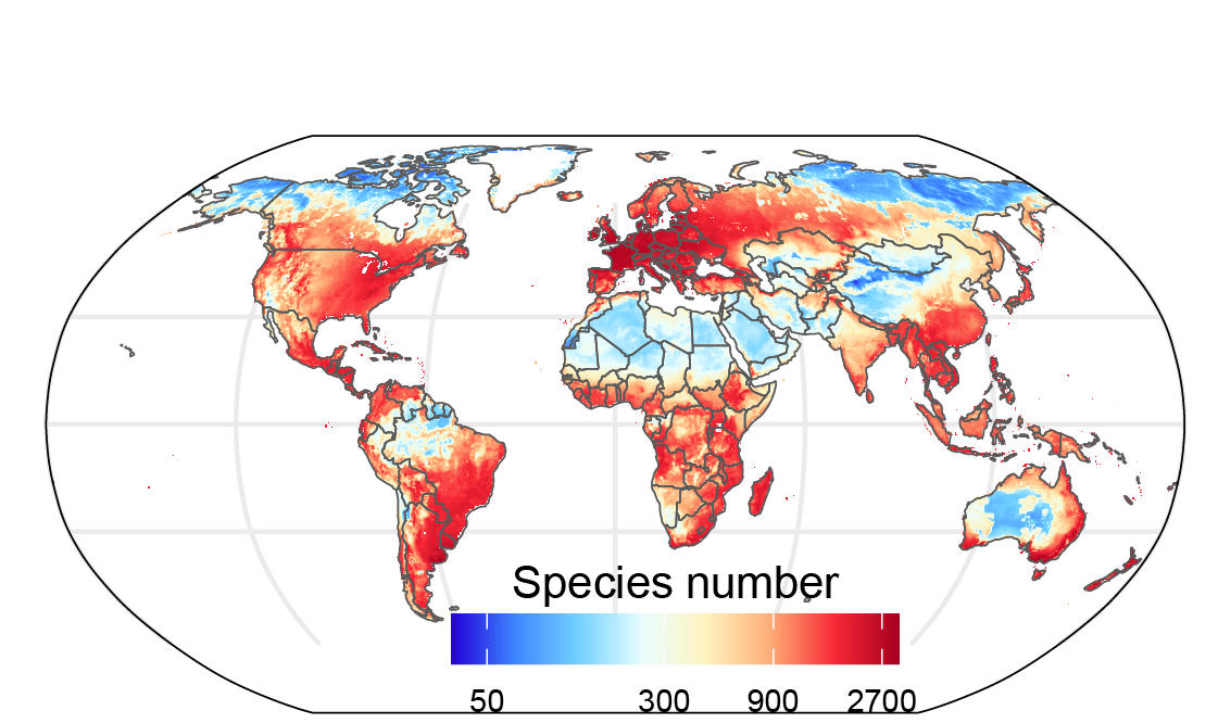
The binary maps for the individual species were then aggregated to calculate the potential alien plant richness in each grid cell under current conditions and future environmental scenarios. The global naturalized plant richness under both current and future scenarios is visualized below, and the corresponding raster data are available for download.

---

Data availability:

Data and R code used to drive the main results in our study are available for download here

---

Data Sources:

Publicly available data sources used in the Project

• GloNAF Database:

  Davis, A. J. S., Dawson, W., Essl, F., Kreft, H., Pergl, J., Pyšek, P.,…van Kleunen, M. (2025). Global Naturalized Alien Flora (GloNAF). Open access data to support research on understanding global plant invasions. https://doi.org/10.5281/zenodo.14696776

• Climatic data:

  Karger, D. N., Conrad, O., Böhner, J., Kawohl, T., Kreft, H., Soria-Auza, R. W.,…Kessler, M. (2017). Climatologies at high resolution for the earth’s land surface areas. Scientific Data, 4(1). https://doi.org/10.1038/sdata.2017.122

• Soil data:

  Poggio, L., de Sousa, L. M., Batjes, N. H., Heuvelink, G. B. M., Kempen, B., Ribeiro, E., & Rossiter, D. (2021). SoilGrids 2.0: producing soil information for the globe with quantified spatial uncertainty. SOIL, 7(1), 217-240. https://soilgrids.org/

• Land use data:

  Hurtt, G. C., Chini, L., Sahajpal, R., Frolking, S., Bodirsky, B. L., Calvin, K.,…Zhang, X. (2020). Harmonization of global land use change and management for the period 850–2100 (LUH2) for CMIP6. Geosci. Model Dev., 13(11), 5425-5464. https://doi.org/10.5194/gmd-13-5425-2020

---

References

• Dong, LJ., Yu, HW. & He, WM. What determines positive, neutral and negative impacts of Solidago canadensis invasion on native plant species richness?. Sci Rep 5, 16804 (2015). https://doi.org/10.1038/srep16804
• POWO. Plants of the World Online. Facilitated by the Royal Botanic Gardens, Kew. Published on the Internet; http://www.plantsoftheworldonline.org/ Retrieved 26 June 2025. (2019).
• Guéguen M, Blancheteau H, Thuiller W. biomod2: Ensemble Platform for Species Distribution Modeling. R package version 4.3-4 (2025). https://biomodhub.github.io/biomod2/
• Hirzel, A. H., Le Lay, G., Helfer, V., Randin, C. & Guisan, A. Evaluating the ability of habitat suitability models to predict species presences. Ecological Modelling 199, 142-152 (2006). https://doi.org/10.1016/j.ecolmodel.2006.05.017

---

Authors Affiliations:

• ¹Division of BioInvasions, Global Change & Macroecology, Department of Botany and Biodiversity Research, University of Vienna, Rennweg 14, Vienna 1030, Austria
• ²Department of Forest Management, Faculty of Forestry, University of Khartoum, North Khartoum, 13314, Sudan
• ³Division of Biodiversity Dynamics & Conservation, Department of Botany and Biodiversity Research, University of Vienna, Rennweg 14, Vienna 1030, Austria
• ⁴Ecology, Department of Biology, University of Konstanz, Universitätsstraße 10, D-78464 Konstanz, Germany
• ⁵Department of Evolution, Ecology and Behaviour, Institute of Infection, Veterinary and Ecological Sciences, University of Liverpool, Liverpool, UK
• ⁶Department of Biology, University of Puerto Rico - Río Piedras, San Juan 00925, Puerto Rico
• ⁷University Grenoble Alpes, University Savoie Mont Blanc, CNRS, LECA, 38000 Grenoble, France
• ⁸Biodiversity, Macroecology & Biogeography, University of Göttingen, Göttingen, Germany
• ⁹Centre of Biodiversity and Sustainable Land Use (CBL), University of Göttingen, Göttingen, Germany
• ¹⁰Campus Institute Data Science (CIDAS), University of Göettingen, Göttingen, Germany
• ¹¹Czech Academy of Sciences, Institute of Botany, Department of Invasion Ecology, CZ-25243 Průhonice, Czech Republic
• ¹²Department of Ecology, Faculty of Science, Charles University, Viničná 7, CZ-12844 Prague, Czech Republic
• ¹³Zhejiang Provincial Key Laboratory of Plant Evolutionary Ecology and Conservation, Taizhou University, Taizhou 318000, China
• ¹⁴Zhejiang Key Laboratory for Restoration of Damaged Coastal Ecosystems, School of Life Sciences, Taizhou University, Taizhou, Zhejiang, 318000, China
• ¹⁵Department of Environmental Science, Radboud Institute for Biological and Environmental Sciences (RIBES), Radboud University, Heyendaalseweg 135, 6525AJ Nijmegen, The Netherlands.
• ¹⁶German Centre of Integrative Biodiversity Research (iDiv) Halle-Jena-Leipzig, Deutscher Platz 5e, DE-04103 Leipzig, Germany
• ¹⁷Institute for Biochemistry and Biology, University of Potsdam, D-14469 Potsdam, Germany

R Code for Species Distribution Modeling (SDM)

This R script shows the steps for generating the Species Distribution Models, including data filtering, pseudo-absence selection, individual model fitting, ensemble modeling, and future forecasting using the BIOMOD2 R package.

# Load required libraries
library(terra)       # For raster and spatial data manipulation
library(biomod2)     # For species distribution modeling
library(tools)       # For file handling
library(dismo)       # For species distribution modeling and analysis
library(sqldf)       # For SQL-like operations on data frames
library(flexsdm)     # For flexible species distribution modeling

# Get command-line arguments (species name)
args = commandArgs(trailingOnly = TRUE)
sp <- args[1]  # First argument is the species name
print(sp)  # Print the species name for debugging

# Set working directory
setwd("*****")

# Read environmental rasters for current and future scenarios
current = rast("bioclim/current/current2.tif")  # Current environmental data
ssp126_100 = list_files_with_exts("bioclim/ssp126_100", exts = "tif")  # Future scenario SSP1-2.6
ssp585_100 = list_files_with_exts("bioclim/ssp585_100", exts = "tif")  # Future scenario SSP5-8.5

# List of environmental data, current and future scenarios
futureenv = c("current/current",
              "ssp126_100/mpi126_100", "ssp126_100/ukesm126_100",
              "ssp585_100/mpi585_100", "ssp585_100/ukesm585_100")

# Read bias file (completness) and mask it to guide the selection of pseudo-absences
biasfile_masked = rast("completness/Meyer_etal_InvCompPlants_111km.tif")

# Read species occurrence data
occ = read.csv(paste0("clean_files/", sp), sep = ",")  # Occurrence data for the species
myCoord = occ[, c('decimalLongitude', 'decimalLatitude')]  # Extract coordinates

# Get species name and clean it
myRespName = unique(occ$species)
myRespName = gsub("-", ' ', myRespName)  # Replace hyphens with spaces
myCoord$id = 1  # Add an ID column

# Filter occurrences based on environmental data
myocc = flexsdm::occfilt_env(myCoord, 'decimalLongitude', 'decimalLatitude', 'id', current, 6)
myCoord = data.frame(myocc[, c('decimalLongitude', 'decimalLatitude')])
myResp = rep(1, nrow(myCoord))  # Response variable (presence = 1)

#Guide the selection of pseudo-absences
# Determine the number of pseudo-absences to generate

  n =  (nrow(occ)


# Format data for BIOMOD2
myBiomodData <- BIOMOD_FormatingData(
  resp.var = myResp,
  expl.var = current,
  resp.xy = myCoord,
  resp.name = paste(myRespName),
  PA.nb.rep = 3,  # Number of pseudo-absence replicates
  PA.sre.quant = 0.025,  # Quantile for SRE
  PA.nb.absences = n,  # Number of pseudo-absences
  PA.strategy = "sre",  # Strategy for pseudo-absence selection
  filter.raster = TRUE
)

# Add a small value to the bias file to avoid zero values
biasfile_masked <- biasfile_masked + 1

# Create SRE (Surface Range Envelope) model
myResp.v <- classify(subset(current, 1), matrix(c(-Inf, Inf, 0), ncol = 3, byrow = TRUE))
myResp.v[cellFromXY(myResp.v, myCoord)] <- 1

sre = bm_SRE(resp.var = myResp.v, expl.var = current, quant = 0.025)
sre = subst(sre, 1, NA)  # Replace 1 with NA in the SRE raster to select pseudo-absences out of the sre

# Mask the bias file with the SRE
biasfile_masked_sre = mask(biasfile_masked, sre)

# Generate pseudo-absences using the bias file
mylist <- list()  # Create an empty list to store pseudo-absences
for (s in 1:3) {
  psa <- terra::spatSample(
    x = biasfile_masked_sre,
    size = n,
    method = "weight",
    na.rm = TRUE,
    as.df = TRUE,
    xy = TRUE
  )[, 1:2]
  mylist[[s]] <- as.data.frame(psa)
}

# Combine pseudo-absences into a single table
PA.tab <- do.call("rbind", mylist)

# Update BIOMOD2 data with new pseudo-absences
myBiomodData@coord <- rbind(myBiomodData@coord[1:length(myResp), ], PA.tab)
myBiomodData@PA.table <- matrix(TRUE, nrow = nrow(myBiomodData@coord), ncol = 3)
myBiomodData@data.env.var <- terra::extract(current, myBiomodData@coord, ID = FALSE)

# Define modeling options
my.opt = bm_ModelingOptions(
  data.type = 'binary',
  models = c('RF', 'GLM', 'GAM', 'GBM'),
  strategy = "user.defined"
)

# Run BIOMOD2 modeling
myBiomodModelOut = BIOMOD_Modeling(
  bm.format = myBiomodData,
  models = c('RF', 'GLM', 'GAM', 'GBM'),
  CV.strategy = 'block',
  metric.eval = c('BOYCE'),
  nb.cpu = 5
)

# Save sigle model evaluation results
write.csv(get_evaluations(myBiomodModelOut), paste0('********', sp, ".csv"), row.names = FALSE)

# Run ensemble modeling
myBiomodEM <- BIOMOD_EnsembleModeling(
  bm.mod = myBiomodModelOut,
  models.chosen = 'all',
  em.algo = c('EMwmean'),
  metric.select = c('BOYCE'),
  nb.cpu = 5
)

# Save variable importance results
write.csv(get_variables_importance(myBiomodEM), paste0('******', sp, ".csv"), row.names = FALSE)

# Project models onto future environmental scenarios
for (h in 1:length(futureenv)) {
  env = rast(paste0("*******", futureenv[h], ".tif"))
  BIOMOD_EnsembleForecasting(
    bm.em = myBiomodEM,
    proj.name = gsub("/", "_", futureenv[h]),
    new.env = env,
    models.chosen = 'all',
    metric.binary = 'BOYCE',
    nb.cpu = 5
  )
  print(h)  # Print progress
}